I’m currently working on another review/instructional paper, this one examining the relationship of paleo-food webs to graph and network theory (along with excursions into combinatorics and counting). Here is a draft of one of the sections. This is a draft! No references, and sketches of figures will be added to the post as they are completed.

GRAPHS

A food web is a summary of interspecific trophic interactions. A mathematical graph is the combination of two sets, commonly written G(V, E), where the elements of E are relationships among the elements of V. Both concepts may be expressed graphically as diagrams of relationships among species or elements, an exercise that makes clear the relationship between the real-world biological system and the abstract mathematical one. The area of mathematics dealing with graphs is known as Graph Theory, familiarity with which proves very useful in the exploration and analysis of not only food webs, but of any real-world system (biological and otherwise) that can be expressed as relationships or interactions among discrete entities. Examples of other systems include networks of genomic interactions, metabolic networks, and phylogenetic trees.

Examine the food webs illustrated in Figure 1. The circles represent species, and the links between them are interspecific interactions. Describing these systems mathematically as G(V,E), the elements of E are relationships among the elements of V. The elements of V are typically referred to as vertices or nodes, and their relationships, or the elements of E, are referred to as edges. Edges are written as pairs of vertices, for example , where and are vertices in G (that is, and ). Species in the food web are therefore nodes, and trophic interactions or links are edges. The first web (Fig. 1A) is a system of non-interacting species 1, 2 and 3. It could function only if embedded within a larger system of species with which these species interacted, or if all three species were autotrophic. Such a graph where no vertices or nodes are connected (E is an empty set) is an unconnected graph, one with some edges is connected (Fig. 1B), while a graph with all vertices connected (Fig. 1C) is a complete graph. Any node to which another is linked is termed its neighbor. Note the alternative representation of a graph as an n by n binary adjacency matrix, where element equals one if an edge connects the two vertices, and zero otherwise.

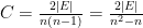
The three graphs would obviously depict food webs with very different implications for the species involved. For example, the density of interactions increases as the number of edges, or |E|, increases. This density is often described simply by the connectance (C) of the graph, standardized as the ratio of the number of edges to the maximum number of edges possible. Each node or species could hypothetically interact with every other species, therefore the number of possible interactions is n(n-1). Note, however, that links would be counted twice, for example {1,2} and {2,1}, so we halve this number. Then

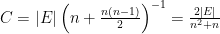
The connectances of Figures 1A-C are therefore zero, 0.333 and 1. We extend this by noting that species may sometimes interact with themselves trophically if individuals are true cannibals. This situation is illustrated in figures as loops, or unit diagonal entries in the adjacency matrix (Fig. 1D). We can now generalize by stating that the connectance of food webs expressed as graphs is measured as

and the connectance of the complete food web in Fig. 1D is therefore 1.

In addition to the overall link density of the graph, or the number of interactions in the food web, we are also interested in the number of interactions per species. This number indicates how trophically specialized or generalized a species is, and is interesting from both evolutionary and ecological perspectives. For example, very specialized species may have stronger coevolutionary interactions with the species to which they are linked, and specialization itself may require temporally extended intervals of stability or high productivity to evolve. Generalized species, on the other hand, could be less susceptible to major perturbations if the intensities of their interactions are distributed broadly among their neighbors. The number of edges or links attached to a node is termed the degree of the node. The simplest cases are those where all nodes are of the same degree, for example Figs. 1A, 1C and 1D. The distribution of links within the graph, or the link distribution, is then single-valued, and may be described as a Dirac delta function or Kronecker’s delta. A slight generalization, where nodes have the same number of links on average, instead of precisely the same degree, leads to the significant development of random graphs and the eventual study of real-world networks.

Next up:Random graphs