Part 1: some toy examples
We start by defining a pure Python function for iterating over a pair of arrays and adding them:
import numpy as np


def addarr(x, y):
    result = np.zeros_like(x)
    for i in range(x.size):
        result[i] = x[i] + y[i]
    return result
n = int(1e6)
a = np.random.rand(n)
b = np.random.rand(n)
%timeit -r 1 -n 1 addarr(a, b)
import numba

addarr_nb = numba.jit(addarr)
%timeit -r 1 -n 1 addarr_nb(a, b)
a and b to addarr could be anything: an array, as expected, but also a list, a tuple, even a Banana, if you’ve defined such a class, and the meaning of the function body is different for each of those types.)
Let’s see what happens the next time we run it:
%timeit -r 1 -n 1 addarr_nb(a, b)
%timeit -r 1 -n 1 a + b
r = np.random.randint(0, 128, size=n).astype(np.uint8)
s = np.random.randint(0, 128, size=n).astype(np.uint8)
%timeit -r 1 -n 1 r + s
%timeit -r 1 -n 1 addarr_nb(r, s)
%timeit -r 1 -n 1 addarr_nb(r, s)
I’m only speculating, but since my clock speed is about 1GHz (I’m writing this on a base Macbook with a 1.1GHz Core-m processor), I suspect that Numba is taking advantage of some SIMD capabilities of the processor, whereas NumPy is treating each array element as an individual arithmetic operation. (If any Numba or NumPy devs are reading this and have more concrete implementation details that explain this, please share them in the comments!)
In this context, I decided to use Numba to do something a little less trivial, as part of my research.
Part 2: Real Numba
%matplotlib inline
import matplotlib.pyplot as plt
plt.rcParams['image.cmap'] = 'gray'
plt.rcParams['image.interpolation'] = 'nearest'
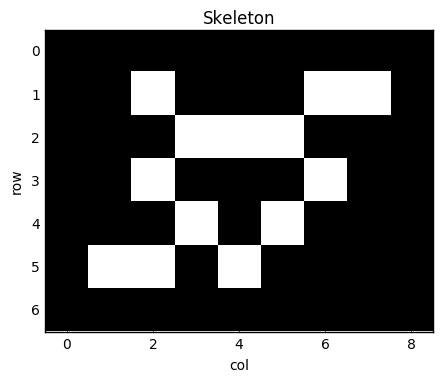
skeleton = np.array([[0, 1, 0, 0, 0, 1, 1],
                     [0, 0, 1, 1, 1, 0, 0],
                     [0, 1, 0, 0, 0, 1, 0],
                     [0, 0, 1, 0, 1, 0, 0],
                     [1, 1, 0, 1, 0, 0, 0]], dtype=bool)
skeleton = np.pad(skeleton, pad_width=1, mode='constant')
fig, ax = plt.subplots(figsize=(5, 5))
ax.imshow(skeleton)
ax.set_title('Skeleton')
ax.set_xlabel('col')
ax.set_ylabel('row')
sparse.coo_matrix format make it very easy to construct such a matrix: we just need an array with the row coordinates and another with the column coordinates.
Because NumPy arrays are not dynamically resizable like Python lists, it helps to know ahead of time how many edges we are going to need to put in our row and column arrays. Thankfully, a well-known theorem of graph theory states that the number of edges of a graph is half the sum of the degrees. In our case, because we want to add the edges twice (once from i to j and once from j to i, we just need the sum of the degrees exactly. We can find this out with a convolution using scipy.ndimage:
from scipy import ndimage as ndi

neighbors = np.array([[1, 1, 1],
                      [1, 0, 1],
                      [1, 1, 1]])

degrees = ndi.convolve(skeleton.astype(int), neighbors) * skeleton
fig, ax = plt.subplots(figsize=(5, 5))
result = ax.imshow(degrees, cmap='magma')
ax.set_title('Skeleton, colored by node degree')
ax.set_xlabel('col')
ax.set_ylabel('row')
cbar = fig.colorbar(result, ax=ax, shrink=0.7)
cbar.set_ticks([0, 1, 2, 3])
cbar.set_label('degree')
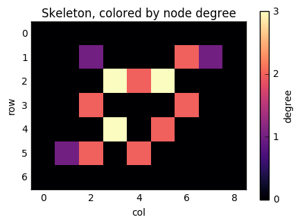
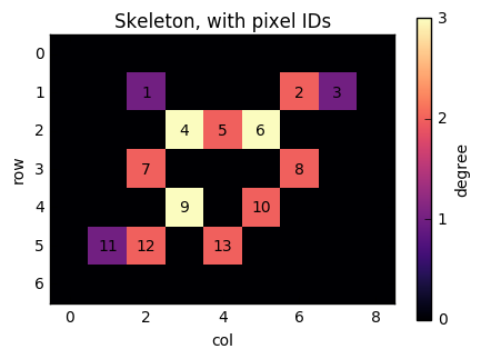
Now, consider the pixel at position (1, 6). It has two neighbours (as indicated by its colour): (2, 5) and (1, 7). If we number the nonzero pixels as 1, 2, …, n from left to right and top to bottom, then this pixel has label 2, and its neighbours have labels 6 and 3. We therefore need to add edges (2, 3) and (2, 6) to the graph. Similarly, when we consider pixel 6, we will add edges (6, 5), (6, 3), and (6, 8).
fig, ax = plt.subplots(figsize=(5, 5))
result = ax.imshow(degrees, cmap='magma')
cbar = fig.colorbar(result, ax=ax, shrink=0.7)
cbar.set_ticks([0, 1, 2, 3])

nnz = len(np.flatnonzero(degrees))
pixel_labels = np.arange(nnz) + 1
for lab, y, x in zip(pixel_labels, *np.nonzero(degrees)):
    ax.text(x, y, lab, horizontalalignment='center',
            verticalalignment='center')

ax.set_xlabel('col')
ax.set_ylabel('row')
ax.set_title('Skeleton, with pixel IDs')
cbar.set_label('degree')
row and col arrays of length exactly np.sum(degrees).
n_edges = np.sum(degrees)
row = np.empty(n_edges, dtype=np.int32)  # type expected by scipy.sparse
col = np.empty(n_edges, dtype=np.int32)
def neighbour_steps(shape):
    step_sizes = np.cumprod((1,) + shape[-1:0:-1])
    axis_steps = np.array([[-1, -1],
                           [-1,  1],
                           [ 1, -1],
                           [ 1,  1]])
    diag = axis_steps @ step_sizes
    steps = np.concatenate((step_sizes, -step_sizes, diag))
    return steps
steps = neighbour_steps(degrees.shape)
print(steps)
Now, we iterate over image pixels, look at neighbors, and populate the row and column vectors.
def build_graph(labeled_pixels, steps_to_neighbours, row, col):
    start = np.max(steps_to_neighbours)
    end = len(labeled_pixels) - start
    elem = 0  # row/col index
    for k in range(start, end):
        i = labeled_pixels[k]
        if i != 0:
            for s in steps:
                neighbour = k + s
                j = labeled_pixels[neighbour]
                if j != 0:
                    row[elem] = i
                    col[elem] = j
                    elem += 1
skeleton_int = np.ravel(skeleton.astype(np.int32))
skeleton_int[np.nonzero(skeleton_int)] = 1 + np.arange(nnz)
%timeit -r 1 -n 1 build_graph(skeleton_int, steps, row, col)
build_graph_nb = numba.jit(build_graph)
%timeit -r 1 -n 1 build_graph_nb(skeleton_int, steps, row, col)
%timeit -r 1 -n 1 build_graph_nb(skeleton_int, steps, row, col)
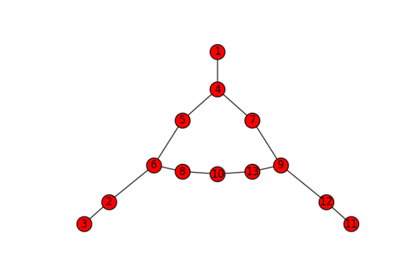
from scipy import sparse
G = sparse.coo_matrix((np.ones_like(row), (row, col))).tocsr()
import networkx as nx

Gnx = nx.from_scipy_sparse_matrix(G)
Gnx.remove_node(0)

nx.draw_spectral(Gnx, with_labels=True)
Conclusion
I hope I’ve piqued your interest in Numba and encouraged you to use it in your own projects. I think the future of success of Python in science heavily depends on JITs, and Numba is a strong contender to be the default JIT in this field.
Note:This post was written using Jupyter Notebook. You can find the source notebook here.

2 thoughts on “Numba in the real world”