
Featured Photo by Luan Rezende
Automatic detection and alarm of abnormal electrocardiogram (ECG aka EKG) events play an important role in an ECG monitor system; however, popular classification models based on standard supervised ML fail to detect abnormal ECG accurately. In this project, we implement an ECG anomaly detection framework based on the recently proposed LSTM Autoencoder.
An autoencoder is a special type of NN that is trained to minimize reconstruction error. The idea is to train an autoencoder on the normal rhythms only, then use it to reconstruct all the data. Our hypothesis is that the abnormal rhythms will have higher reconstruction error. We will then classify a rhythm as an anomaly if the reconstruction error surpasses a fixed threshold.
An LSTM Autoencoder is an implementation of an autoencoder for sequence data using an Encoder-Decoder LSTM architecture.
Objective – To Detect abnormal beats in ECG waveforms
We will train an autoencoder to detect anomalies on the ECG5000 dataset. This dataset contains 5,000 Electrocardiograms, each with 140 data points.
Contents:
- Background
- The Dataset
- LSTM NN Workflow
- Preparation
- EDA
- LSTM RNN Encoder
- Training RNN
- Predictions
- Summary
- Explore More
- Infographic
Background
- An electrocardiogram (ECG or EKG) is a test that checks how your heart is functioning by measuring the electrical activity of the heart. With each heart beat, an electrical impulse (or wave) travels through your heart. This wave causes the muscle to squeeze and pump blood from the heart.
- Assuming a healthy heart and a typical rate of 70 to 75 beats per minute, each cardiac cycle, or heartbeat, takes about 0.8 seconds to complete the cycle. Frequency: 60–100 per minute (Humans) Duration: 0.6–1 second (Humans).
The Dataset
- The dataset contains 5,000 Time Series examples (obtained with ECG) with 140 timesteps. Each sequence corresponds to a single heartbeat from a single patient with congestive heart failure.
We have 5 types of hearbeats (classes):
- Normal (N)
- R-on-T Premature Ventricular Contraction (R-on-T PVC)
- Premature Ventricular Contraction (PVC)
- Supra-ventricular Premature or Ectopic Beat (SP or EB)
- Unclassified Beat (UB).
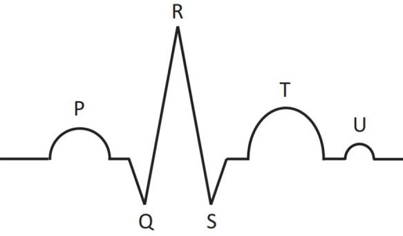
Schematic representation of main parts of the ECG signal for one cardiac cycle: P, T, U waves and QRS complex, consisting of Q, R, and S peaks.
The dataset was originally published in “Goldberger AL, Amaral LAN, Glass L, Hausdorff JM, Ivanov PCh, Mark RG, Mietus JE, Moody GB, Peng C-K, Stanley HE. PhysioBank, PhysioToolkit, and PhysioNet: Components of a New Research Resource for Complex Physiologic Signals. Circulation 101(23)”. The dataset was pre-processed in two steps: (1) extract each heartbeat, (2) make each heartbeat equal length using interpolation. This dataset was originally used in paper “A general framework for never-ending learning from time series streams”, DAMI 29(6). After that, 5,000 heartbeats were randomly selected. The patient has severe congestive heart failure and the class values were obtained by automated annotation.
LSTM NN Workflow
- Preparation Phase
- Exploratory Data Analysis (EDA)
- Building the LSTM Encoder
- Training and Running NN Model
- Detect ECG anomalies with THRESHOLD
- Plot true and reconstructed ECG anomalies
Preparation
We begin by setting the working directory YOURPATH
import os
os.chdir(‘YOURPATH’)
os. getcwd()
Let’s download and unzip the input dataset
unzip ECG5000.zip
Let’s import the key libraries
import seaborn as sns
import matplotlib as mpl
import numpy as np
from scipy.io.arff import loadarff
import pandas as pd
import matplotlib.pyplot as plt
from sklearn.model_selection import train_test_split
import torch
from scipy.io.arff import loadarff
from sklearn.metrics import confusion_matrix, classification_report
from glob import glob
import time
import copy
import shutil
from torch import nn, optim
import torch.nn.functional as F
from torchvision import datasets,transforms,models
%matplotlib inline
%config InlineBackend.figure_format =’retina’
sns.set(style=’whitegrid’,palette=’muted’,font_scale=1.2)
HAPPY_COLORS_PALETTE = [“#01BEFE”, “#FFDD00”, “#FF7D00”, “#FF006D”, “#ADFF02”, “#8F00FF”]
sns.set_palette(sns.color_palette(HAPPY_COLORS_PALETTE))
mpl.rcParams[‘figure.figsize’] = 12, 8
RANDOM_SEED = 42
np.random.seed(RANDOM_SEED)
torch.manual_seed(RANDOM_SEED)
Let’s define the torch device
device =torch.device(‘cuda’ if torch.cuda.is_available() else ‘cpu’)
and read the train and test data using loadarff
with open(‘ECG5000_TRAIN.arff’) as f:
raw_data = loadarff(f)
train = pd.DataFrame(raw_data[0])
with open(‘ECG5000_TEST.arff’) as f:
raw_data1 = loadarff(f)
test = pd.DataFrame(raw_data1[0])
Let’s check the test dataset structure
test.head()
with 5 rows × 141 columns.
Let’s create the dataframe
df =train.append(test)
df.head()
EDA
Let’s perform some data preparations for NN model training
df.shape
(5000, 141)
df=df.sample(frac=1.0)
CLASS_NORMAL = 1
class_names =[‘Normal’,’PVC’, ‘R on T’,’SP’,’UB’]
new_columns = list(df.columns)
new_columns[-1] = ‘target’
df.columns = new_columns
df.head()
5 rows × 141 columns
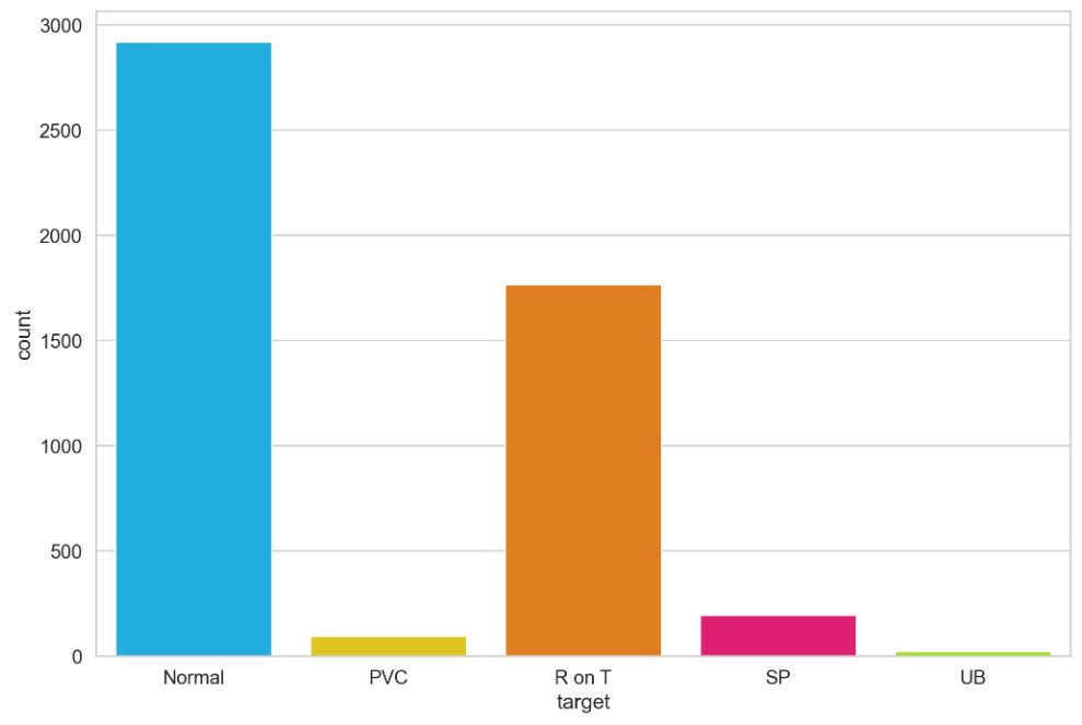
df.target.value_counts()
b'1'    2919
b'2'    1767
b'4'     194
b'3'      96
b'5'      24
Name: target, dtype: int64
Let’s plot the counts of 5 classes (target)
ax = sns.countplot(df.target)
ax.set_xticklabels(class_names);
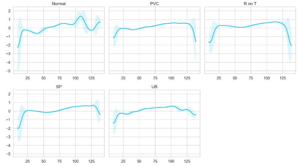
We can also plot the averaged time-series data for each class
def plot_time_series_class(data, class_name, ax, n_steps=10):
time_series_df = pd.DataFrame(data)
smooth_path = time_series_df.rolling(n_steps).mean()
path_deviation = 2 * time_series_df.rolling(n_steps).std()
under_line = (smooth_path – path_deviation)[0]
over_line = (smooth_path + path_deviation)[0]
ax.plot(smooth_path, linewidth=2)
ax.fill_between(
path_deviation.index,
under_line,
over_line,
alpha=.125
)
ax.set_title(class_name)
classes = df.target.unique()
fig, axs = plt.subplots(
nrows=len(classes) // 3 + 1,
ncols=3,
sharey=True,
figsize=(14, 8)
)
for i, cls in enumerate(classes):
ax = axs.flat[i]
data = df[df.target == cls] \
.drop(labels=’target’, axis=1) \
.mean(axis=0) \
.to_numpy()
plot_time_series_class(data, class_names[i], ax)
fig.delaxes(axs.flat[-1])
fig.tight_layout();
Let’s select Normal b’1′ class for training purposes
normal_df = df[df.target==b’1′].drop(labels=’target’,axis =1)
normal_df.shape
(2919, 140)
The input to our training process is as follows
anomaly_df = df[df.target !=b’1′].drop(labels=’target’,axis =1)
anomaly_df.shape
(2081, 140)
Let’s split our data
train_df, val_df = train_test_split(
normal_df,
test_size=0.15,
random_state=RANDOM_SEED
)
val_df, test_df = train_test_split(
val_df,
test_size=0.33,
random_state=RANDOM_SEED
)
Let’s create the input training dataset
def create_dataset(df):
sequences = df.astype(np.float32).to_numpy().tolist()
dataset = [torch.tensor(s).unsqueeze(1).float() for s in sequences]
n_seq, seq_len, n_features = torch.stack(dataset).shape
return dataset, seq_len, n_features
train_dataset, seq_len, n_features = create_dataset(train_df)
val_dataset, , = create_dataset(val_df)
test_normal_dataset, , = create_dataset(test_df)
test_anomaly_dataset, , = create_dataset(anomaly_df)
LSTM RNN Encoder
Let’s build the Encoder/Decoder representing 2 separate layers of the LSTM RNN
class Encoder(nn.Module):
def init(self, seq_len, n_features, embedding_dim=64):
super(Encoder, self).init()
self.seq_len, self.n_features = seq_len, n_features
self.embedding_dim, self.hidden_dim = embedding_dim, 2 * embedding_dim

self.rnn1 = nn.LSTM(
  input_size=n_features,
  hidden_size=self.hidden_dim,
  num_layers=1,
  batch_first=True
)
# Initializing the hidden numbers of layers
self.rnn2 = nn.LSTM(
input_size=self.hidden_dim,
hidden_size=embedding_dim,
num_layers=1,
batch_first=True
)
def forward(self, x):
x = x.reshape((1, self.seq_len, self.n_features))
x, (_, _) = self.rnn1(x)
x, (hidden_n, _) = self.rnn2(x)

return hidden_n.reshape((self.n_features, self.embedding_dim))
class Decoder(nn.Module):
def init(self, seq_len, input_dim=64, n_features=1):
super(Decoder, self).init()
self.seq_len, self.input_dim = seq_len, input_dim
self.hidden_dim, self.n_features = 2 * input_dim, n_features

self.rnn1 = nn.LSTM(
  input_size=input_dim,
  hidden_size=input_dim,
  num_layers=1,
  batch_first=True
)
Using a dense layer as an output layer
self.rnn2 = nn.LSTM(
  input_size=input_dim,
  hidden_size=self.hidden_dim,
  num_layers=1,
  batch_first=True
)

self.output_layer = nn.Linear(self.hidden_dim, n_features)
def forward(self, x):
x = x.repeat(self.seq_len, self.n_features)
x = x.reshape((self.n_features, self.seq_len, self.input_dim))
x, (hidden_n, cell_n) = self.rnn1(x)
x, (hidden_n, cell_n) = self.rnn2(x)
x = x.reshape((self.seq_len, self.hidden_dim))

return self.output_layer(x)
The RecurrentAutoencoder = Encoder + Decoder is given by
class RecurrentAutoencoder(nn.Module):
def init(self, seq_len, n_features, embedding_dim=64):
super(RecurrentAutoencoder, self).init()
self.encoder = Encoder(seq_len, n_features, embedding_dim).to(device)
self.decoder = Decoder(seq_len, embedding_dim, n_features).to(device)
def forward(self, x):
x = self.encoder(x)
x = self.decoder(x)
return x
Let’s build our RNN model
model = RecurrentAutoencoder(seq_len, n_features, 128)
model = model.to(device)
Training RNN
Let’s train and evaluate the LSTM model
def train_model(model, train_dataset, val_dataset, n_epochs):
optimizer = torch.optim.Adam(model.parameters(), lr=1e-3)
criterion = nn.L1Loss(reduction=’sum’).to(device)
history = dict(train=[], val=[])
best_model_wts = copy.deepcopy(model.state_dict())
best_loss = 10000.0
for epoch in range(1, n_epochs + 1):
    model = model.train()
    train_losses = []
    for seq_true in train_dataset:
        optimizer.zero_grad()
        seq_true = seq_true.to(device)
        seq_pred = model(seq_true)
        loss = criterion(seq_pred, seq_true)
        loss.backward()
        optimizer.step()
        train_losses.append(loss.item())
val_losses = []
model = model.eval()
with torch.no_grad():
    for seq_true in val_dataset:
        seq_true = seq_true.to(device)
        seq_pred = model(seq_true)
        loss = criterion(seq_pred, seq_true)
        val_losses.append(loss.item())

train_loss = np.mean(train_losses)
val_loss = np.mean(val_losses)

history['train'].append(train_loss)
history['val'].append(val_loss)

if val_loss < best_loss:
    best_loss = val_loss
    best_model_wts = copy.deepcopy(model.state_dict())

print(f'Epoch {epoch}: train loss {train_loss} val loss {val_loss}')

model.load_state_dict(best_model_wts)
return model.eval(), history
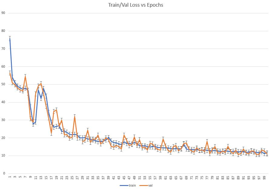
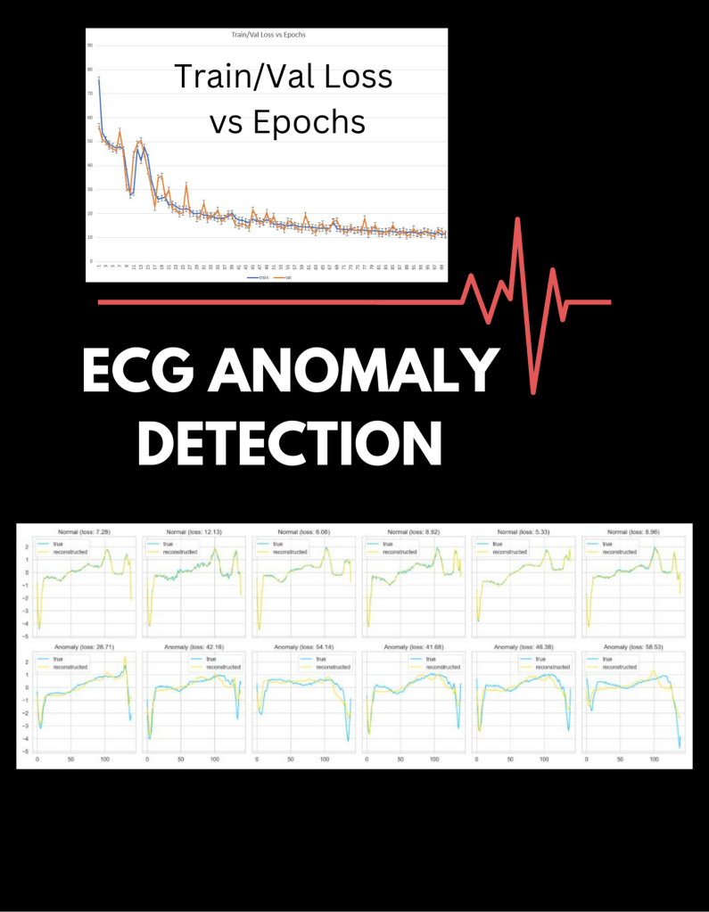
model,history = train_model(model,train_dataset,val_dataset,n_epochs=100)
Let’s plot training/validation Loss vs Epochs
Predictions
Let’s perform our predictions
def predict(model, dataset):
predictions, losses = [], []
criterion = nn.L1Loss(reduction=’sum’).to(device)
with torch.no_grad():
model = model.eval()
for seq_true in dataset:
seq_true = seq_true.to(device)
seq_pred = model(seq_true)
loss = criterion(seq_pred, seq_true)
predictions.append(seq_pred.cpu().numpy().flatten())
losses.append(loss.item())
return predictions, losses
and plot the corresponding histograms of predicted losses
predictions, pred_losses = predict(model, test_normal_dataset)
sns.distplot(pred_losses, bins=50, kde=True);
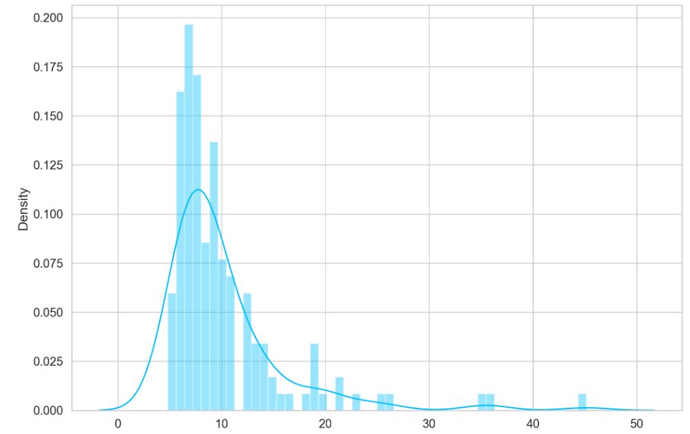
Let’s define the threshold value
THRESHOLD = 20
and check correct normal predictions
correct = sum(l <= THRESHOLD for l in pred_losses)
print(f’Correct normal predictions: {correct}/{len(test_normal_dataset)}’)
Correct normal predictions: 137/145
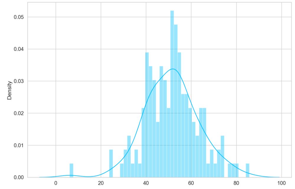
Let’s look at the test normal dataset
anomaly_dataset = test_anomaly_dataset[:len(test_normal_dataset)]
predictions, pred_losses = predict(model, anomaly_dataset)
sns.distplot(pred_losses, bins=50, kde=True);
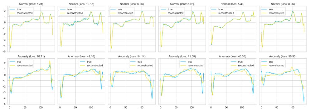
Finally, let’s plot our predictions for both normal and anomaly data
def plot_prediction(data, model, title, ax):
predictions, pred_losses = predict(model, [data])
ax.plot(data, label=’true’)
ax.plot(predictions[0], label=’reconstructed’)
ax.set_title(f'{title} (loss: {np.around(pred_losses[0], 2)})’)
ax.legend()
fig, axs = plt.subplots(
nrows=2,
ncols=6,
sharey=True,
sharex=True,
figsize=(22, 8)
)
for i, data in enumerate(test_normal_dataset[:6]):
plot_prediction(data, model, title=’Normal’, ax=axs[0, i])
for i, data in enumerate(test_anomaly_dataset[:6]):
plot_prediction(data, model, title=’Anomaly’, ax=axs[1, i])
fig.tight_layout();
Summary
- ECG data can provide a wealth of information about a patient’s health.
- Accurate detection sudden abnormal ECG is an important procedure in EWS ECG; however, even experienced clinicians struggle to distinguish normal from anomalous EGCs in cases when the differences are subtle.
- The proposed Autoencoder (AE) improves the detection rate of abnormal ECG while ensuring high accuracy of predictions.
- Test results on ECG5000 data show that the AE reconstruction error discriminates between normal and anomalous beats for further assessment by clinicians or analysis through additional methods.
Explore More
Anomaly Detection using AutoEncoders – A Walk-Through in Python
Beginner-friendly ECG anomaly detection using Autoencoders
Chapter 9 – Anomaly Detection – ECG pulse detection.ipynb
LSTM Autoencoder for Anomaly Detection for ECG data
Abnormal ECG detection based on an adversarial autoencoder
Infographic
Make a one-time donation
Make a monthly donation
Make a yearly donation
Choose an amount
Or enter a custom amount
Your contribution is appreciated.
Your contribution is appreciated.
Your contribution is appreciated.
DonateDonate monthlyDonate yearly